PDLP

Abstract

This paper presents a synchronized system of the pool-based spot and perpetual futures DEX with built-in dynamic LP hedging and MEV protection.

Background

DEX evolution

Since the introduction of the “xyk” model pioneered by Uniswap V1/V2, the on-chain liquidity market structure has significantly evolved. While groundbreaking, the monolithic approach of constant product AMM had limitations, such as high slippage and inefficient liquidity usage. As the space matured, new DEX architectures emerged, tailored to specific use cases, such as the Stableswap invariant from Curve Finance, the Request-for-Quote (RFQ) system from 0x, batch auctions from CoWSwap, and the concentrated liquidity model of Uniswap V3. Each closes its own unique market needs by improving liquidity providers' user experience in terms of flexibility and/or capital efficiency.

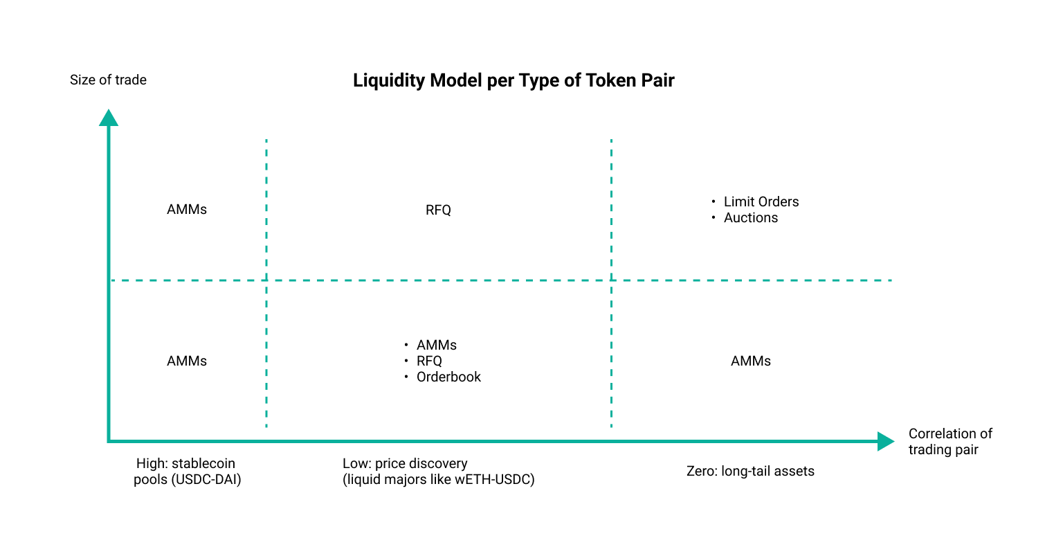
These advancements mirror the evolution of blockchain technology itself. As Ethereum was the first to separate consensus and application logic, enabling developers to create dApps without building their own blockchains but instead leveraging a shared security model, the latest DEX models began to separate liquidity provision from clearing and settlement. In this regard, Uniswap V3 custom liquidity ranges provide LPs greater flexibility in terms of expressing their portfolio preferences and boosting capital efficiency while still receiving shared trade flow from aggregated liquidity curves.

Similarly, as Ethereum moved to a modular scalability approach by separating execution and settlement/validation via applying rollups + data availability layer model, we are witnessing further trends of externalizing management from financial infrastructure in both DEXes and lending markets architectural landscapes. Namely, the Coincidence-of-Wants (CoWS) mechanism from CoW Swap and the emergence of intent-centric architectures like CoW Protocol intents/hooks and Uniswap V4 hooks in the decentralized exchanges DeFi segment.

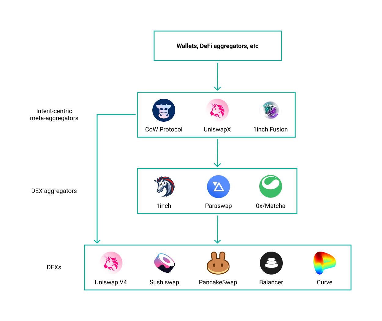
This approach enables LPs to express their preferences and requirements through intents, which can include parameters like price, size, and customized trading strategies via conditional orders. The routing problem is being outsourced to external parties - a network of solvers or fillers who compete to satisfy these intents by sourcing liquidity for optimal order execution. This separation allows LPs to focus on defining their desired trading strategies and risk profiles without restrictions to follow any specific rules, such as Uniswap V3 invariant curve, enabling ultimate flexibility in adapting strategies and algorithms to constantly evolving market conditions. While inclusion into a competitive solvers network ensures preserving trade flow by tapping into the liquidity and user base of established meta-aggregators.

Application-specific lending

At the same time, we witness the growing popularity of the new class of decentralized derivatives exchanges powered by the pool-based architecture. Namely, GMX’s GM pools, Jupiter’s JLP, and Hyperliquid’s HLP products are powered by the perpetual demand lending pools (PDLPs) that lend pool assets to perpetual traders. Where users who want passive yield deposit multiple assets into the ETF-like weighted pool and their assets are lent out to collateralize perp positions.

For example, a trader opens up a 5x leveraged long position by providing 1x collateral and the pool lends out the remaining 4x.

The loan is closed when either:

1. A trader pays back accrued fees and returns their collateral
2. A trader is liquidated, returning the pool’s assets back

Unlike other DeFi lending protocols, there is no liquidation bonus and the collateral just goes back to the pool. This is an important difference and when assets don’t leave the pool, lending protocol knows where the borrowed assets are and can reclaim the exact amount that was lent out upon liquidation (application-specific lending).

Powered by the Target Weight Mechanism (TWM), this nature is similar to the CFMMs, but as assets don’t leave the pool, the only moving part is oracle-based prices that affect portfolio weight distribution. This construction is much easier to hedge compared to the CFMMs, as amounts don’t change and we only need to hedge the delta of the underlying assets.

As a result of new passive yield vaults quickly emerged that provide liquidity for the JLP pool and dynamically hedge it with perpetual futures on external exchanges, such as Drift.

Another notable example of an application-specific lending protocol is Panoptic. The protocol applies the same application-specific lending theme to Uniswap V3 LP tokens. The core idea is that a concentrated range position resembles a short put option, and by lending that LP token to an options buyer, Panoptic effectively converts passive range liquidity into convex option-like pay-offs for long speculators.

Recently, Chitra et al. (2025) provided the first structural model of perpetual-demand lending pools. Their analysis:

1. Formalizes the Target-Weight Mechanism that keeps the pool’s asset mix close to predetermined weights
2. Characterizes the arbitrage loop that restores those weights whenever oracle prices move
3. Derives the equilibrium funding-rate curve that balances trader demand with pool utilization
4. Produces a closed-form mean-variance hedge that maximizes the pool’s Sharpe ratio.

Building on those results, the optimal hedge for a pool that lends out an asset vector $l$ and faces price covariance $\Sigma$ is:

where

• $f$ – the (annualized) fee rate earned on the lent inventory (funding rate),
• $\gamma$ – the vault’s risk-tolerance slider,
• $\Delta$ – the pool’s post-trade delta, i.e. the spot exposure that remains after the Target-Weight swap.

The first term sizes a short that monetizes the fee stream while capping variance; the second neutralizes the pool’s raw long. Chitra et al. show that as long as

adding $\pi^{\star}$ can only improve the pool’s Sharpe ratio and never increase its volatility by more than a factor of four.

For a pool that lends only WETH and keeps the remainder in USDC, the covariance matrix collapses to a single variance term $\sigma^2_{WETH}$:

• $l$ - WETH currently on loan
• $R_{WETH}$ - pool inventory after the user-facing swap/deposit/withdraw
• $f$ - fee rate quoted by the lending module (annual funding rate)
• $\sigma^2$ - rolling variance of daily WETH returns (EWMA)
• $\gamma$ - risk-tolerance slider (clipped to the Sharpe-safe ceiling $\gamma_{max} = \frac{fl}{\sigma^2 R_{WETH}}$)

The pool is perfectly delta-neutral when $\pi^* = -R_{WETH}$ (set $\gamma = \gamma_{max}$), smaller $\gamma$ lets it run a measured long to harvest more carry.

These closed-form expressions remove the need for iterative inventory management and make on-chain, block-by-block hedging feasible. Based on these findings, we will construct our perpetual demand lending pool with a built-in LP hedging powered by Euler lending protocol and Uniswap V4 hooks.

Mechanism Design

Design Objective

Create an on-chain mechanism of the pool-based perpetual futures exchange that:

1. Enables leveraged trading.
2. Optimized for the efficient Uniswap LP hedging - accept collateral in USDC and quote assets (BTC, ETH, etc) for both long and short positions*.
3. Maintain target PDLP portfolio value distribution.
4. Implement atomic hedge inside every pool-mutating transaction, such as Pool $(R, l)$ + Hedge $(\pi)$ has constant delta $|\partial V / \partial P|$
5. Preserves MEV resistance - the hedge must be settled (or the tx is reverted) before the block is final.
6. Keeps Sharpe floor intact $fl \geq \gamma \sigma^2 R$

*On the upside Uniswap LPs receive USDC from USDC → ETH swaps and on the downside ETH from ETH → USDC swaps.

Built-in PDLP hedging

To achieve built-in PDLP dynamic hedging we will use looping on Euler lending protocol. This way, instead of using external derivatives CEX/DEX venues, we will employ the same EVM state for higher capital-efficiency and atomicity.

Where the flow will be the following:

1. Split initial USDC portfolio into 2 parts:
   1. USDC: $\text{totalCollateralUSDC} = w\cdot V$
   2. ETH: $\text{totalCollateralETH} = (1-w)\frac{V}{P}$, where $P$ is the ETH/USDC price
2. Supply both of them as collateral on Euler lending protocol
3. Take a debt $\text{debtETH} = k \cdot \text{totalCollateralETH}$
4. Swap $d\cdot \text{debtETH} \cdot P$ and add to the totalCollateralUSDC
5. Supply $(1-d)\cdot \text{debtETH}$ into the totalCollateralETH

Effectively creating a leveraged long position with the portfolio value:

With the parameters $w=0.5, k=1, d=0.5$ - the initial LTV will be at 33.3%.

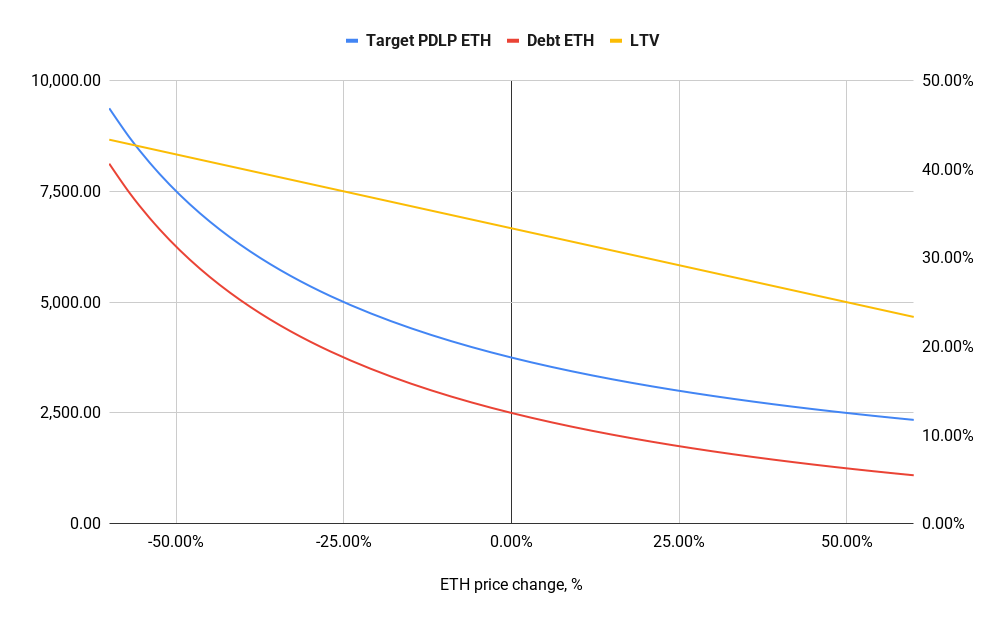
As the underlying asset price change, our totalCollateralUSDC will remain the same but we will adjust our debtETH to preserve the constant delta of our portfolio by keeping $\text{totalCollateralETH}-\text{debtETH}$ constant.

In our configuration, the Target Weight Mechanism will target the equal PDLP portfolio distribution between ETH and USDC reserves, such as

To achieve this, we will gradually adjust our collateral/debt state:

As for trading and position management, because of the PDLP as a leveraged long position with a constant delta - we will apply momentum-based approach rather than typical mean-reversion approach when PDLP open an opposite position.

In our case, new long position will increase our ETH exposure and debt, thus pushing LTV higher (which goes down on the upside). While with the short positions - we will repay our ETH debt pushing LTV down to reduce our liquidation risk on the downside. Targeting this way constant LTV ratio to minimize liquidation risk by applying funding rate mechanism.

Long position:

1. Ping the latest oracle update
2. Open
   1. Accept USDC collateral
   2. Increase debtETH by $\frac{\text{collateralUSDC} \cdot \text{leverage}}{P_{AMM}}$
   3. Move newly issued debt to the ETH balance.
3. Close
   1. Repay debtETH with the totalCollateralETH
   2. Settle USDC PnL with the user.

Short position:

1. Ping the latest oracle update
2. Open
   1. Accept USDC collateral
   2. Repay ETH debt by the $\frac{\text{collateralUSDC} \cdot \text{leverage}}{P_{AMM}}$ by using our totalCollateralETH funds.
3. Close
   1. Increase debtETH with the totalCollateralETH funds.
   2. Settle USDC PnL with the user.

Internal Price

The internal trade price $P_{AMM}$ is determined based on the latest oracle price and the concentrated liquidity model of Uniswap V3.

1. Ping oracle
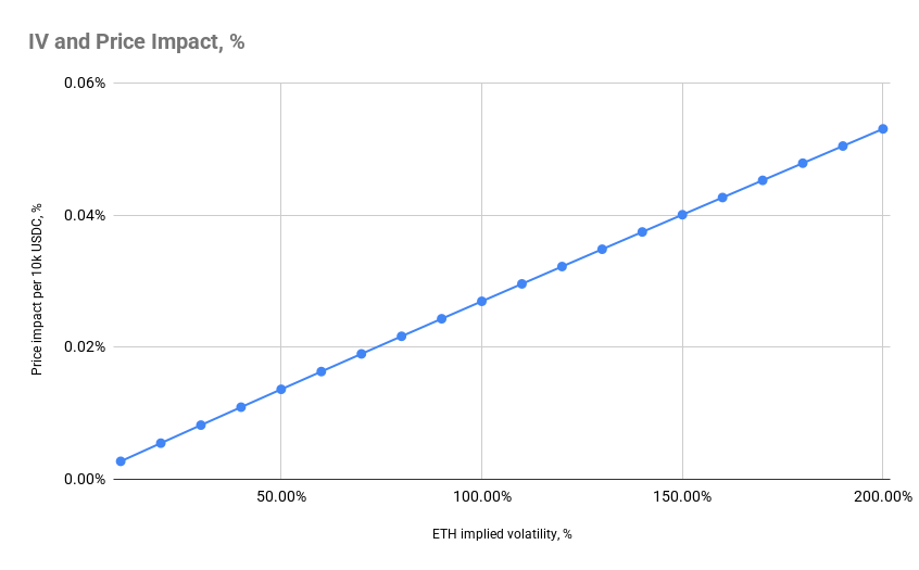
2. Dynamic liquidity - calculate liquidity based on the Uniswap function getLiquidityForAmount0(uint160 sqrtPriceAX96, uint160 sqrtPriceBX96, uint256 amount0)
3. Inputs:
   1. amount0 - our total USDC collateral
   2. sqrtPriceAX96 and sqrtPriceBX96 - lower and upper boundaries calculated based on the expected weekly price change obtained from the underlying asset implied volatility: $Range = P_{oracle}(1\pm \frac{IV}{\sqrt{52}})$

For example, with the ETH/USDC oracle price 2000 and IV 60% the boundaries will be [1833, 2166]. While with the IV 80% the boundaries will be [1778, 2221].

Stability mechanism

1. Scope and safety envelope

To maintain system stability and healthy risk-management, we limit maximum open interest rate between long and short positions based on the total portfolio market exposure:

Open interest on one side of the book can never exceed the vault’s net long ETH.

2. Funding rate

Upside scenario

Price ↑ ⇒ vault’s LTV falls (debt/value shrinks). If traders keep adding longs the pool must borrow still more ETH, pushing LTV back up. → Funding should rise to tilt new flow toward shorts and stabilize LTV.

Downside scenario

Price ↓ ⇒ LTV rises. More shorts arrive with ETH collateral (basis-trade), the pool repays debtETH and LTV drops. → Funding can fall (even flip negative) to favour new longs and stop LTV from undershooting.

Thus funding is the vault’s feedback valve: make longs expensive when you need shorts, make shorts expensive when you need longs.

As our PDLP keeps a constant net delta, the Sharpe-ratio bound from Chitra et al.

collapses to a linear rule in the forward variance $\sigma^2$.

To stay above that line—and to pull the health-factor back whenever the vault takes on too much borrow leverage—we quote a funding rate with only two moving parts:

Key point: traders must always receive at least the USDC money-market rate plus a volatility spread; otherwise it will be not enough to incentivize traders to open a new positions on our platform.

Because $\Delta_{\text{pool}}$ is fixed, the volatility term alone already fulfills Chitra’s Sharpe condition; the LTV kicker is a purely defensive layer that throttles leverage back under the cap without active intervention.

This mechanism yields a self-contained, MEV-safe PDLP: atomic hedging keeps Δ constant, utilization and LTV are steered by a two-factor funding curve, and the Sharpe condition is enforced on-chain every funding tick.

Trading fee

• Flat rate $\phi = 5$ bp (0.05 %) charged on notional each time a position is opened or closed.
• Collection method
  • USDC collateral – fee is debited in USDC and immediately added to the pool’s USDC reserves.
  • Underlying asset collateral (ETH) – fee is debited in ETH and added to the pool’s ETH reserves.
• Accounting – because the fee is swept straight into collateral, TVL and the pool’s net equity rise deterministically with volume and automatically included in the upcoming hedge update.

Structured Vaults

The proposed PDLP design with a built-in LP hedging was specifically constructed for the precise, atomic impermanent loss hedging of the liquidity provision on spot DEXes. This way, we can create a directional (targets underlying asset outperformance) and delta-neutral (targets USD yield) vaults that can capture spot trading fees while staying protected from impermanent loss.

Directional vault

The goal is to create a synthetic portfolio that outperforms the underlying asset (BTC, ETH, etc) by providing liquidity on Uniswap V4 and dynamically hedging its impermanent loss with long perps on PDLP.

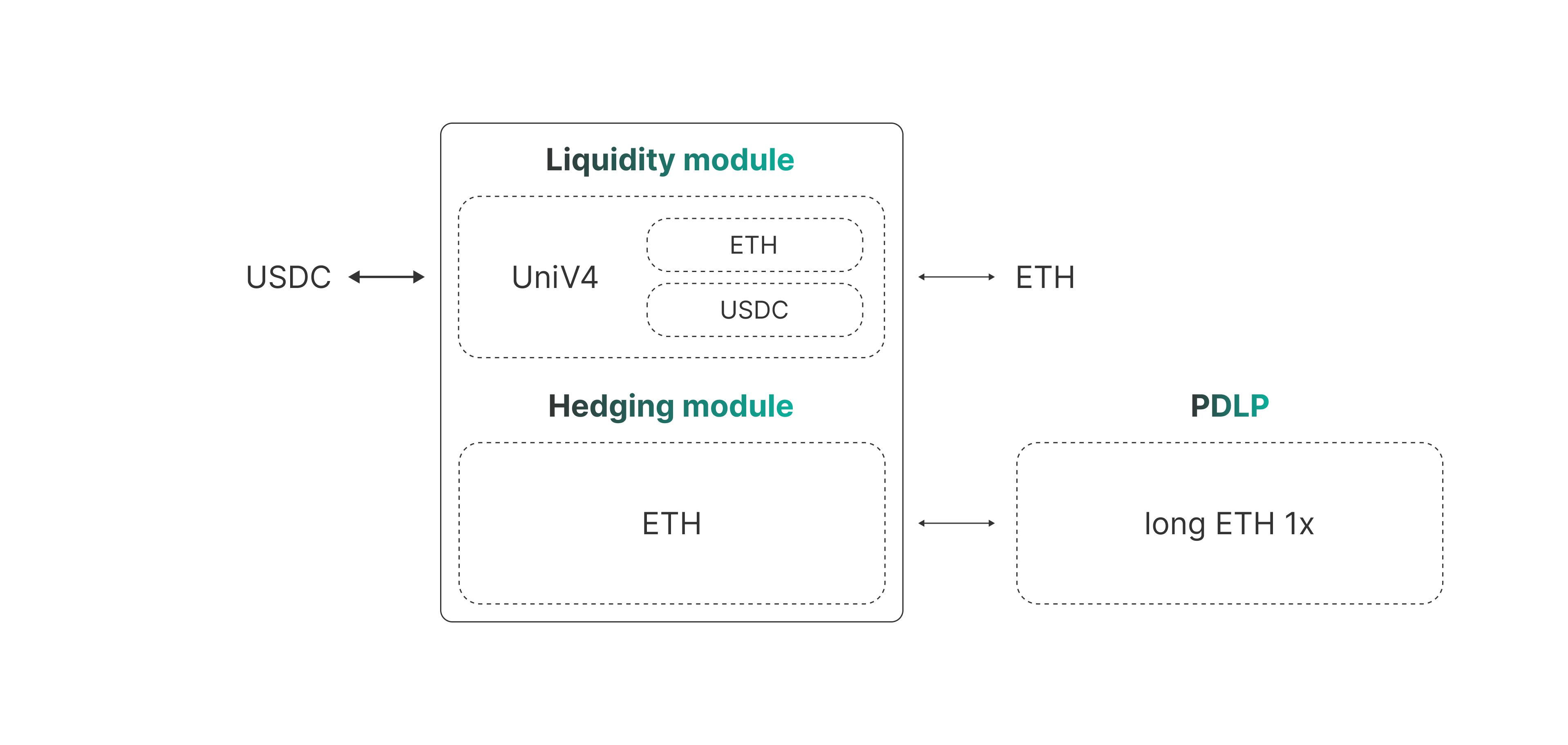
The flow:

1. Accept ETH for deposits
2. Convert 50% to USDC
3. Add liquidity to the Uniswap V4 ETH-USDC pool
4. For the USDC → ETH swap:
   1. Receive USDC
   2. Calculate ETH output based on the Uniswap math.
   3. Send ETH to the user
   4. Use ETH in hedging module to adjust long position on PDLP.
5. For the ETH → USDC swap:
   1. Receive ETH
   2. Calculate USDC output based on the Uniswap math.
   3. Send USDC to the user
   4. Use ETH in hedging module to adjust long position on PDLP.

This way, our directional vault effectively executes a tokenized spot-perp arbitrage in which we sell spot ETH while simultaneously buying long ETH perp (hedge our impermanent loss). Where our yield is the difference between the spot trading fees and execution costs.

Delta-neutral vault

The goal is to create a portfolio that earns trading fees independently from the market conditions by providing liquidity on Uniswap and dynamically hedging its price exposure with short perps on PDLP. Mirroring vault to the directional one by introducing which we also optimize execution costs for both directional and delta-neutral vaults.

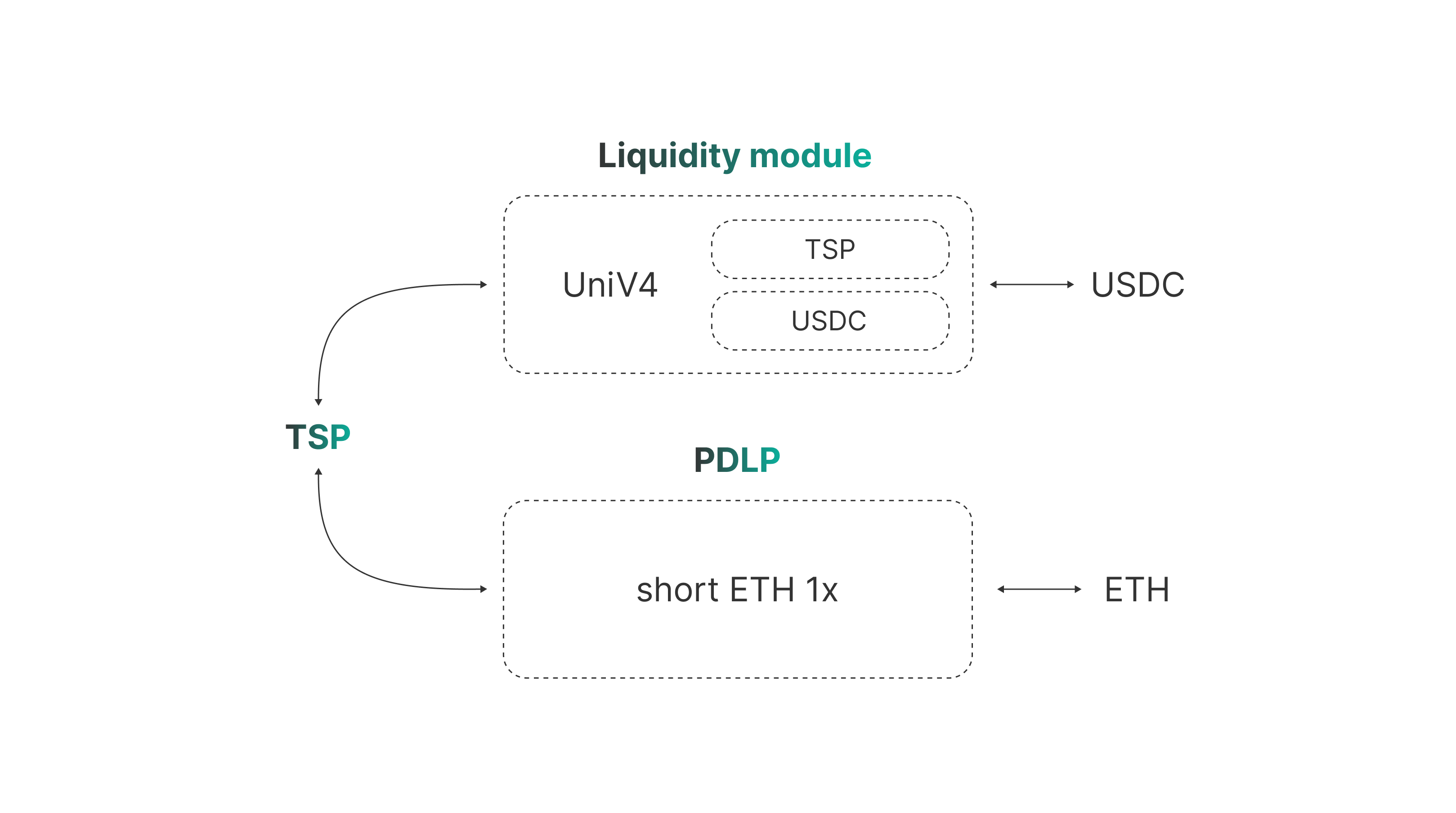
The flow:

1. Accept USDC for deposits
2. Convert 50% to ETH
3. Basis trade:
   1. Use received ETH to open a short 1x position
   2. Tokenize it as a TSP
4. Match tokenized 1x short perp position against USDC in the concentrated liquidity pool on Uniswap V4 (TSP-USDC)
5. For the USDC → ETH swap:
   1. Receive USDC
   2. Swap it for the tokenized short position
   3. Redeem tokenized short position for the underlying asset (ETH)
   4. Send ETH to the user
6. For the ETH → USDC swap:
   1. Receive ETH
   2. Use it to open a tokenized 1x short perp position
   3. Swap received tokenized short position for the USDC
   4. Send USDC to the user

Liquidity Orchestrator

The Orchestrator stitches the two vaults and the Uniswap V4 / CoWSwap solver mesh into a single, MEV-safe pipeline.

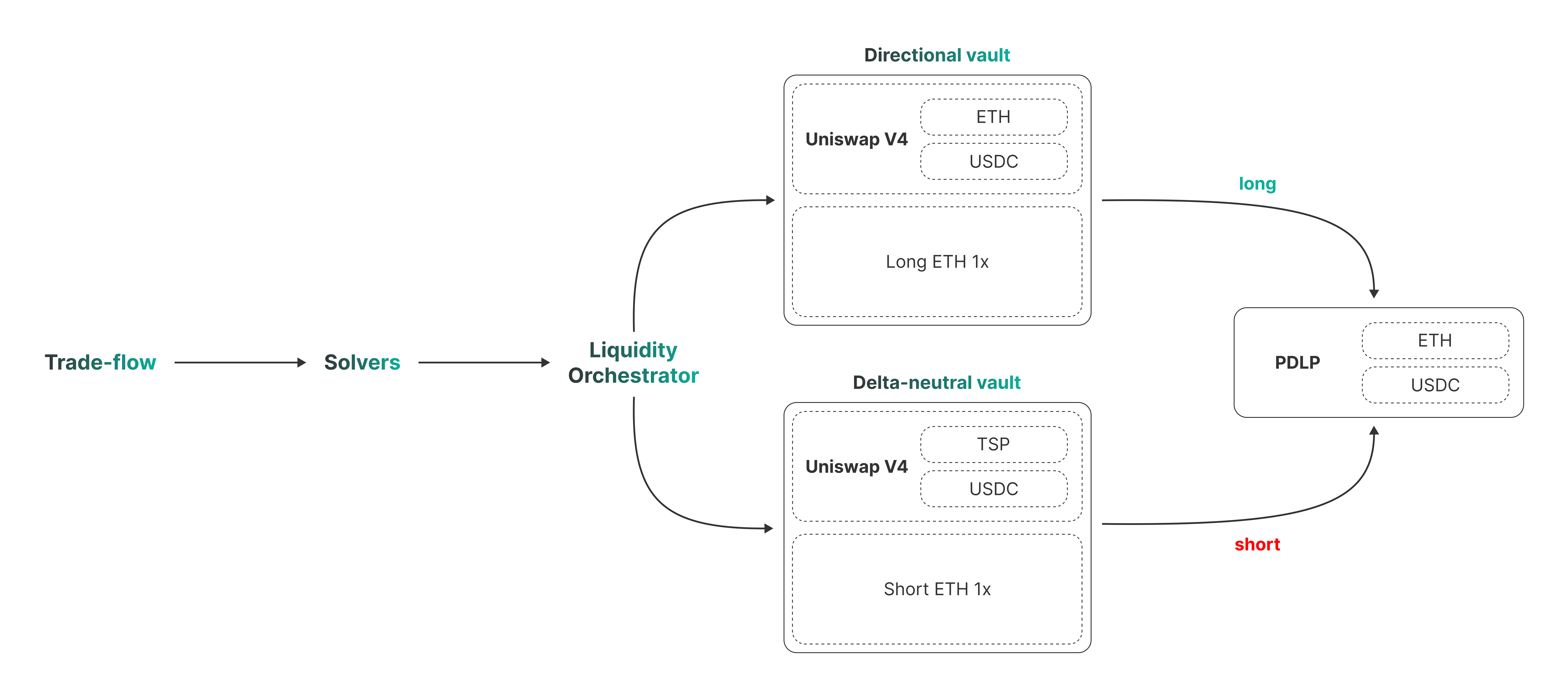
The flow:

1. Intents - users submit trades as a signed intents to the network of solvers of meta-aggregators
2. Liquidity Orchestrator - solvers send these intents to the Liquidity Orchestrator (LO).
3. Oracle ping – LO pulls the latest price and pushes it to the perp-pricing contract.
4. Batching / coincidence-search – intents are grouped to
   1. check for liquidations
   2. net as much long vs short flow as possible by routing through directional and delta-neutral vaults → lower price-impact
   3. respect maxOIΔ, Sharpe floor, and target LTV.
   4. accrue the funding rate
5. Single dispatch – the whole batch is executed atomically.

Embedding the LO in the Uniswap V4 / CoWSwap solver network leverages their no-arbitrage guarantee: if an external CEX/DEX price drift makes an arbitrage possible, a solver routes that trade through our PDLP contract. The hedge auto-fires, so the pool’s payoff curve stays constant-leverage and MEV-protected.

Profitability analysis

PDLP

For a pool that targets constant-delta, LP’s yield constitutes of the:

1. USDC interest rate from the yield-bearing collateral on Euler.
2. Perps trading fees

Both can be represented as a function of implied volatility with empirical values around $\frac{\sigma^2}{8}$ for the USDC interest rate (higher IV indicates more demand for decentralized leverage) and around $\frac{\sigma^2}{4}$ for trading fees paid for hedging.

For example, with a utilization 50%, target delta 0.25, and IV 60%, PDLP depositors can expect:

1. For the -60% underlying price change (ETH/USDC from $4k → $1.6k):
   • PnL: $-60\% \cdot 0.25 = -15\%$
   • Fees: $\approx 13.43\%$
   • Total: $\approx -1.58\%$
2. For the +60% underlying price change (ETH/USDC from $2k → $3.2k):
   • PnL: $+60\% \cdot 0.25 = +15\%$
   • Fees: $\approx 21.38\%$
   • Total: $\approx 36.38\%$

Resulting in a convex payoff obtained from the volatility harvesting strategy. Because both fee flow and the USDC lending yield quadratically scale up with IV while downside price exposure remains capped at $\delta = 0.25$, the pool behaves like a convex volatility harvester:

• in quiet markets LPs still collect the baseline USDC rate;
• as volatility rises, cash-flows grow quadratically (interest and fees), quickly outpacing the linear mark-to-market drag of an adverse price move;
• on rallies the constant long-delta turns the same fee stack into leveraged upside.

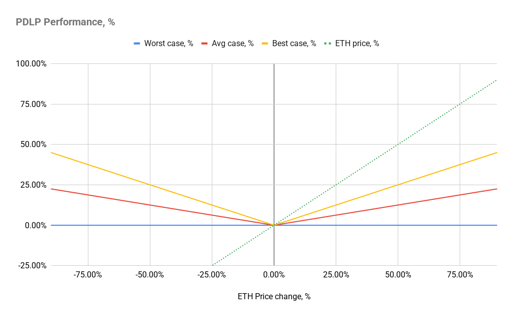
Below is how those cash-flows translate into total vault returns across a full price cycle and correspondent expected yield based on the volatility regimes:

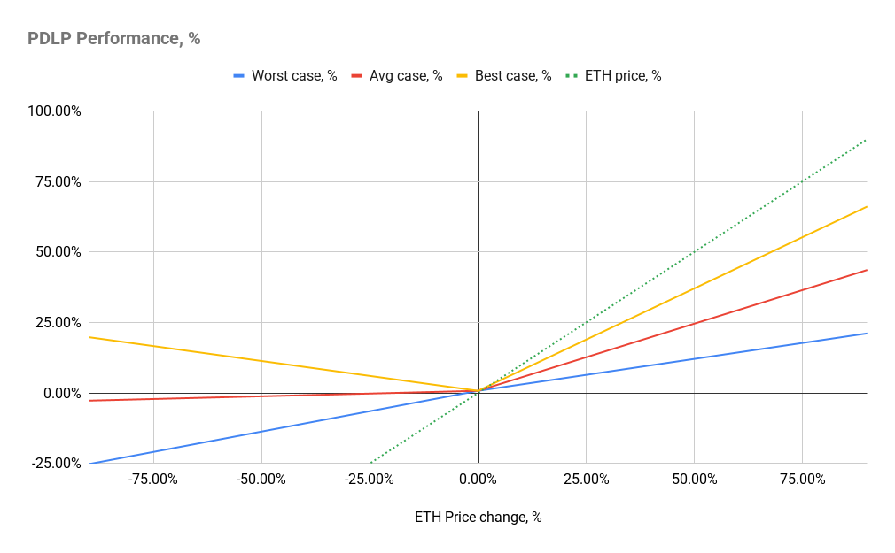
• Green - underlying asset price change
• Blue - worst case PDLP: every trader is on the right side of the move, so LPs surrender the full 0.25 × price drift while still collecting only the baseline vol-linked cash-flows.
• Red - average case: long and short flow balance 50 : 50. Half the positions lose and recycle fees to winners, so LPs pockets the interest rate and trading fees, preserving the constant pool delta.
• Yellow - best case: every trader was wrong; the vault keeps all fee income and also harvests their losses, producing the steepest convex payoff.

The wedge illustrates the earlier point on convex volatility harvesting with ETH beta:

• Downside is capped at 0.25 delta and can be fully covered by the volatility-linked cash-flows at typical mid-volatility regimes.
• Upside stacks leveraged spot gain while collecting interest rates and trading fees which tends to increase on upside movements.

Atomic hedging, the max-OI envelope and the funding-rate/LTV feedback loop lock these pay-offs in without relying on external keepers or off-chain inventory. Inclusion into the shared trade-flow from the solver networks (Uniswap / CoWSwap) provide us with a sustainable trading fee source of income paid for hedging (no need for the individual traders).

The result is a self-rebalancing vault that offers LPs a vol-linked yield with convex ETH beta, rather than the concave profile of traditional AMMs, all while preserving on-chain Sharpe guarantees from the Chitra framework.

Note: PDLP is a very flexible structure which parameters can be adjusted to control for the delta and expected performance. For example, by adding a short leg or setting $k=2$ - we can transform our PDLP into a structure that even in the worst case is just a delta-neutral strategy, while average case yielding $\sigma^2/2$ offering attractive risk-adjusted returns.

Finally, following Chitra’s framework - delta can be calculated dynamically rather than statically for future performance optimization tailored for a different volatility regimes and market trends.

Vaults

Where $r^S$ is spot trading fees, $r^H$ is hedging execution cost, and $f$ is the funding rate.

The total expected spot trading fees $r^S$ is around $\frac{\sigma^2}{2}$ from which we pay half of the fees for the PDLP hedging execution and also funding rate for position preserving.

The expected APY for different market regimes varies from $\sigma^2/8$ to $\sigma^2/4$. For example, with the IV at 80%, LPs can expect the following APY:

On average, 12% APY for directional and delta-neutral vaults for IV = 80% market regime.

Conclusion

Lumis turns the perpetual-demand-lending idea into a self-hedging, solver-native liquidity layer in which:

• a looped-short on Euler fixes the pool’s net delta (Δ ≈ 0 or 0.25, set by the single knob k);
• a two-factor funding curve - USDC floor + LTV-kicker - pays the gamma bill and drags leverage back inside the risk envelope;
• Yield from trading fees and interest rate scale linearly with implied volatility $\sigma^2$, giving LPs a payoff that is convex to volatility and beta-positive to the underlying asset (ETH).

Directional and delta-neutral vaults reverse which side of the funding leg they monetize, giving LPs a clear menu of risk flavours that both average to c. 12 % APY at IV = 80 %.

Future Work

1. Adaptive $\Delta$ / dynamic $\gamma$

We used fixed $k$ (hence delta) for simplicity. In reality Sharpe-optimal γ drifts with σ, funding basis and pool utilization $u$.

For this we need adaptive controllers that solve for γ* each epoch and translate it into a new k without large rebalance costs. This controller will reinforce the Chitra inequality with real-time estimates and let the contract solve for the γ that maximizes expected Sharpe each funding tick. Requires on-chain optimization that is both gas-cheap and MEV-safe.

2. Multi-asset extension

A basket (e.g., ETH, wBTC, etc) dilutes idiosyncratic risk and broadens perp flow, but $\Sigma^{-1}l$ in Chitra’s hedge becomes full-rank.

It will require to generalize the Euler loop to an n-vector hedge that uses a covariance matrix. Possible area of research is also a cross-asset funding curves that compensate for covariance, not just variance.

3. Atomic derivatives

By synchronizing spot and derivatives layers via liquidity orchestrator, we can design a custom derivatives that dynamically adjust its price exposure following the pre-specified rules.

← Back to research